
Abstract
This paper examines short-term price reactions after one-day abnormal price changes and whether they create exploitable profit opportunities in various financial markets. Statistical tests confirm the presence of overreactions and also suggest that there is an “inertia anomaly”, i.e. after an overreaction day prices tend to move in the same direction for some time. A trading robot approach is then used to test two trading strategies aimed at exploiting the detected anomalies to make abnormal profits. The results suggest that a strategy based on counter-movements after overreactions does not generate profits in the FOREX and the commodity markets, but in some cases it can be profitable in the US stock market. By contrast, a strategy exploiting the “inertia anomaly” produces profits in the case of the FOREX and the commodity markets, but not in the case of the US stock market.
1 Introduction
The efficient market hypothesis (EMH) is one of the cornerstones of financial economics (Fama 1965). Its implication is that there should not be any exploitable profit opportunities in financial markets. However, the empirical literature has documented the presence of a number of so-called “market anomalies”, i.e. price behaviour that appears to create abnormal profit opportunities.
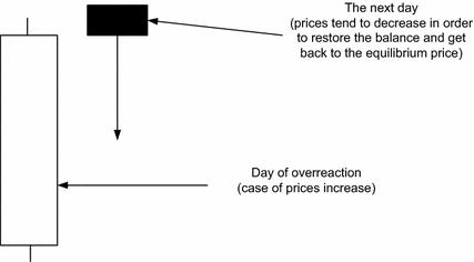
One of the most famous stock market anomalies is the so-called overreaction hypothesis detected by De Bondt and Thaler (1985), who showed that investors tend to give excessive weight to recent relative to past information when making their portfolio choices. A special case of the overreaction hypothesis is short-term price reactions after one-day abnormal price changes. Empirical studies on various financial markets show that after such price changes there are bigger contrarian price movements than after normal (typical) daily fluctuations (Atkins and Dyl 1990; Bremer and Sweeney 1991; Bremer et al. 1997; Cox and Peterson 1994; Choi and Jayaraman 2009; etc).
This paper provides new evidence on the overreaction anomaly by analysing both price counter-movements and movements in the direction of the overreaction and comparing them to those after normal days. First, we carry out t tests to establish whether the data generation process of prices is the same after days of overreaction and typical days. We show that short-term overreactions cause the emergence of patterns in price behaviour, i.e. temporary market inefficiencies that could result in extra profit opportunities. Then we use a trading robot method to examine whether or not trading strategies based on the detected statistical anomalies are profitable, i.e. whether price overreactions are simply statistical phenomena or can also be seen as evidence against the EMH. The analysis is carried out for various financial markets: the US stock market (the Dow Jones index and two companies included in this index), FOREX (EURUSD, USDJPY, GBPCHF, AUDUSD) and commodity markets (Gold, Oil).
The remainder of this paper is organised as follows. Section 2 briefly reviews the existing literature on the overreaction hypothesis. Section 3 outlines the methodology followed in this study. Section 4 discusses the empirical results. Section 5 offers some concluding remarks.
2 Literature Review
There is a vast empirical literature on the EMH. Kothari and Warner (2006) reviewed over 500 studies providing evidence in support of this paradigm. However, as pointed out by Ball (2009), there is also plenty of evidence suggesting the presence of market anomalies apparently inconsistent with EMH such as over- and under-reactions to information flows, volatility explosions and seasonal yield bursts, yield dependence on different variables such as market capitalisation, dividend rate, and market factors, etc. Over- or under-reactions are significant deviations of asset prices from their average values during certain periods of time (Stefanescu et al. 2012).
The overreaction hypothesis was first considered by De Bondt and Thaler (DT 1985), following the work of Kahneman and Tversky (1982), who had shown that investors overvalue recent relative to past information. The main conclusions of DT were that the best (worst) performing portfolios in the NYSE over a three-year period tended to under (over)-perform over the following three-year period. Overreactions are associated with irrational behaviour of investors who overreact to news arrivals. This leads to significant deviations of asset prices from their fundamental value. Such overreactions normally lead to price corrections. An interesting fact, mentioned by DT, is an asymmetry in the overreaction: its size is bigger for undervalued than for overvalued stocks. DT also reported the existence of a “January effect”, i.e. overreactions tend to occur mostly in that month.
Subsequent studies on the overreaction hypothesis include Brown et al. (1988), who analysed NYSE data for the period 1946–1983 and reached similar conclusions to DT; Zarowin (1989), who showed the presence of short-term market overreactions; Atkins and Dyl (1990), who found overreactions in the NYSE after significant price changes in one trading day, especially in the case of falling prices; Ferri and Min (1996), who confirmed the presence of overreactions using S&P 500 data for the period 1962–1991; Larson and Madura (2003), who used NYSE data for the period 1988–1998 and also showed the presence of overreactions, as did Clements et al. (2009).
Overreactions have also been found in other stock markets, including Spain (Alonso and Rubio 1990), Canada (Kryzanowski and Zhang 1992), Australia (Brailsford 1992; Clare and Thomas 1995), Japan (Chang et al. 1995), Hong-Kong (Akhigbe et al. 1998), Brazil (DaCosta 1994; Richards 1997), New Zealand (Bowman and Iverson 1998), China (Wang et al. 2004), Greek (Antoniou et al. 2005), Turkey (Vardar and Okan 2008) and Ukraine (Mynhardt and Plastun 2013). Some evidence is also available for other types of markets, such as the gold market (Cutler et al. 1991) and the option market (Poteshman 2001).
A few studies have examined whether such anomalies give rise to profit opportunities. In particular, Jegadeesh and Titman (1993) developed a trading strategy based on an algorithm consisting in undertaking transactions in the opposite direction to the previous movement at a monthly frequency. They found that such a strategy generates a 12% profit per year. A similar strategy, but at a weekly frequency, was developed by Lehmann (1990), and was found to be equally profitable.
3 Data and Methodology
We analyse the following daily series: for the US stock market, the Dow Jones index and stocks of two companies included in this index (Microsoft and Boeing—for the trading robot analysis we also add Wal Mart and Exxon); for the FOREX, EURUSD, USDJPY and GBCHF (for the trading robot analysis also AUDUSD); for commodities, Gold and Oil. The sample period covers the period from January 2002 till the end of September 2014 (for the trading robot analysis the period is 2012–2014).
3.1 Statistical Tests
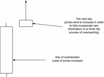
First we carry out Student’s t tests to confirm (reject) the presence of anomalies after overreactions. To provide additional evidences in favor of the tested hypotheses we use ANOVA analysis. Also, to overcome normal distribution limitations we carry out Kruskall–Wallis tests. Then we apply the trading robot approach to establish whether detected anomalies create exploitable profit opportunities. According to the classical overreaction hypothesis, an overreaction should be followed by a correction, i.e. price counter-movements, and bigger than after normal days. If one day is not enough for the market to incorporate new information, i.e. to overreact, then after one-day abnormal price changes one can expect movements in the direction of the overreaction bigger than after normal days.
Therefore the following two hypotheses will be tested:
- H1 :
-
Counter-reactions after overreactions differ from those after normal days.
- H2 :
-
Price movements after overreactions in the direction of the overreaction differ from such movements after normal days.


The null hypothesis is in both cases that the data after normal and overreaction days belong to the same population.
We analyse short-term overreactions, so the period of analysis is 1 day (one trading session). The parameters characterising price behaviour over such a time interval are maximum, minimum, open and close prices. In most studies price movements are measured as the difference between the open and close price. For the purposes of the current study the daily return is measured as the difference between the maximum and minimum prices during the day. It is more appropriate, because we are interested in extreme points of the daily fluctuations. The use of maximum–minimum instead of open-close allows us to analyse the full amplitude of the daily price changes. This is calculated as:
where \(R_i \) is the % daily return, \(High_i \) is the maximum price, and \(Low_i \) is the minimum price for day i.
We consider the following definition of “overreaction”:
where k-the number of standard deviations used to identify overreaction,
\(\bar{{R}}_n \) is the average size of daily returns for period n
and \(\delta _n \) is the standard deviation of daily returns for period n
The next step is to determine the size of the price movement during the next day. For Hypothesis 1 (the counter-reaction or counter-movement assumption), we measure it as the difference between the next day’s open price and the maximum deviation from it in the opposite direction to the price movement in the overreaction day.
If the price increased, then the size of the counter-reaction is calculated as:
where \(cR_{i+1} \) is the counter-reaction size, and \(Open_{i + l} \) is the next day’s open price.
If the price decreased, then the corresponding definition is:
In the case of Hypothesis 2 (movement in the direction of the overreaction), either Eqs. (6) or (5) is used depending on whether the price has increased or decreased.
Two data sets (with \(cR_{i+1} \) values) are then constructed, including the size of price movements after normal and abnormal price changes respectively. The first data set consists of \(cR_{i+1} \) values after 1-day abnormal price changes. The second contains \(cR_{i+1} \) values after a day with normal price changes. The null hypothesis to be tested is that they are both drawn from the same population.
3.2 Trading Robot Analysis
The trading robot approach considers the short-term overreactions from a trader’s viewpoint, i.e. whether it is possible to make abnormal profits by exploiting the overreaction anomaly. The trading robot simulates the actions of a trader according to an algorithm (trading strategy). This is a programme in the MetaTrader terminal that has been developed in MetaQuotes Language 4 (MQL4) and used for the automation of analytical and trading processes. Trading robots (called experts in MetaTrader) allow to analyse price data and manage trading activities on the basis of the signals received.
We examine two trading strategies:
-
Strategy 1 (based on H1) This is based on the classical short-term overreaction anomaly, i.e. the presence the abnormal counter-reactions the day after the overreaction day. The algorithm is constructed as follows: at the end of the overreaction day financial assets are sold or bought depending on whether abnormal price increases or decreased respectively have occurred. An open position is closed if a target profit value is reached or at the end of the following day (for details of how the target profit value is defined see below).
-
Strategy 2 (based on H2) This is based on the non-classical short-term overreaction anomaly, i.e. the presence the abnormal price movements in the direction of the overreaction the following day. The algorithm is built as follows: at the end of the overreaction day financial assets are bought or sold depending on whether abnormal price increases or decreases respectively have occurred. Again, an open position is closed if a target profit value is reached or at the end of the following day.
In order to avoid data-snooping bias and artificial fitting of certain parametersFootnote 1 we adopt the following testing procedure.
-
1.
We use a base period (data from 2013) to obtain the optimal parameters for the behaviour of asset prices (an example of such optimisation is reported in “Appendix 1”).
-
2.
We test the trading strategy with the optimal parameters on the base period (2013 data) and two independent (non-optimised) periods (2012 and 2014) to see whether it is profitable (an example can be found in “Appendix 2”).
-
3.
We perform continuous testing for the period 2012–2014 to obtain average results for the trading strategy.
-
4.
The results of continuous trading are used to assess the effectiveness of the strategy. If total profits from trading are >0 and the number of profitable trades is >50%, and the results are rather stable for different periods, then we conclude that there is a market anomaly and it is exploitable.
To make sure that the results we obtain are statistically different from the random ones we carry out t tests. We chose this approach instead of carrying out z tests because the sample size is less than 100. A t test compares the means from two samples to see whether they come from the same population. In our case the first is the average profit/loss factor of one trade applying the trading strategy, and the second is equal to zero because random trading (without transaction costs) should generate zero profit.
The null hypothesis (H0) is that the mean is the same in both samples, and the alternative (H1) that it is not. The computed values of the t test are compared with the critical one at the 5% significance level. Failure to reject H0 implies that there are no advantages from exploiting the trading strategy being considered, whilst a rejection suggests that the adopted strategy can generate abnormal profits.
Example of the t test results are reported in Table 1.
As it can be seen, H0 is confirmed, which implies that the trading simulation results are not statistically different from the random ones and therefore this trading strategy is not effective and there is no exploitable profit opportunity.
The results of the trading strategy testing and some key data are presented in the “Report” in “Appendix 2”. The most important indicators given in the “Report” are:
-
Total net profit: this is the difference between “Gross profit” and “Gross loss” measured in US dollars. We used marginal trading with the leverage 1:100, therefore it is necessary to invest $1000 to make the profit mentioned in the Trading Report. The annual return is defined as Total net profit/100, so, for instance, an annual total net profit of $100 represents a 10% annual return on the investment;
-
Profit trades: % of successful trades in total trades;
-
Expected payoff: the mathematical expectation of a win. This parameter represents the average profit/loss per trade. It is also the expected profitability/unprofitability of the next trade;
-
Total trades: total amount of trade positions;
-
Bars in test: the number of past observations modelled in bars during testing.
The results are summarised in the “Graph” section of the “Report”: this represents the account balance and general account status considering open positions. The “Report” also provides full information on all the simulated transactions and their financial results. The following parameters affect the profitability of the trading strategies (the next section explains how they are set):
-
Criterion for overreaction (symbol: sigma_dz): the number of standard deviations added to the mean to form the standard day interval;
-
Period of averaging (period_dz): the size of data set on which base mean and standard deviation are counted;
-
Time in position (time_val): how long (in hours) the opened position has to be held;
-
Expected profit per trade or Take Profit (profit_koef): the size of profit expected to result from a trade, measured as:
$$\begin{aligned} {\text {Take Profit}}={\text {profit}}\_{\text {koef}}\;^*\,{\text {sigma}}\_{\text {dz}}; \end{aligned}$$ -
Maximum amount of losses per trade or Stop Loss (stop): the size of losses the trader is willing to incur in a trade, defined as follows:
$$\begin{aligned} {\text {Stop Loss}} ={\text {stop}}\;^*\,{\text {sigma}}\_{\text {dz}}. \end{aligned}$$
4 Empirical Results
The first step is to set the basic overreaction parameters/criterions by choosing the number of standard deviations (sigma_dz) to be added to the average to form the “standard” day interval for price fluctuations and the averaging period to calculate the mean and the standard deviation(symbol: period_dz).
For this purpose we used the Dow Jones index data for the period 1987–2012. The number of abnormal returns detected in the period 1987–2012 is reported in Table 2.
As can be seen, both parameters (averaging period and number of standard deviations added to the mean) affect the number of detected anomalies. Changes in the averaging period only have a small effect (the difference between the results when the period considered is 5 and 30 respectively is less than 10%). By contrast, each additional standard deviation significantly decreases the number of observed abnormal returns (by 50% for each additional sigma). Therefore 2–4% of the full sample (the number of abnormal returns in the case of 3 sigmas) is not sufficiently representative to draw conclusions. That is why we set the parameter sigma_dz equal to 1. Evidence that this is true holds not only in case of the Dow Jones index data but also for the other financial assets as is presented in Table 3.
To make sure that this choice is reasonable in practice we test the trading strategy based on overreactions with a different set of parameters (see “Appendix 3”). The results provide evidence in favour of 1 as an appropriate value for the sigma_dz parameter. Student’s t tests of short-term counter-reactions carried out for the Dow Jones index over the period 1987–2012 (see Table 4) suggest that the optimal averaging periods are 20 and 30 (the corresponding t statistics are significantly higher than for other averaging periods), and thus the t tests are also performed for these.
The results for H1 are presented in “Appendices 6–8” and are summarized in Table 5.
In the case of the commodity markets H1 is rejected for Oil (that is, we obtain evidence in favor of anomaly presence) but cannot be rejected for Gold for both averaging periods. The results from testing Hypothesis 1 for the US stock markets are stable for the two averaging periods (20 and 30) and confirm the presence of a statistical anomaly in the price dynamics in the US stock market after short-term overreactions.
The results from testing Hypothesis 1 for the FOREX are not as stable as those for the US stock market. No anomaly is detected for the EURUSD (for both periods of averaging), whilst one is observed in the behaviour of GBPCHF (for both averaging periods). The USDJPY results are sensitive to the choice of the averaging period (an anomaly is found with an averaging period of 20, but not of 30).
Overall, it appears that in the case of H1 the longer the averaging period is, the bigger is the probability of anomaly detection. H1 cannot be rejected for the US stock market (in all cases) and in some cases for the FOREX (USDJPY and GBPCHF) and commodity (Oil) markets when the averaging period is 30. Therefore the classical short-term counter-movement after an overreaction day is confirmed in many cases, especially with an averaging period_dz \(=\) 30. The only exceptions are Gold and EURUSD.
The results for H2 are presented in “Appendices 9–11” and are summarized in Table 6.
Hypothesis 2 can be rejected in most cases for the commodity markets (the only exception is Gold with an averaging period of 20). The results from testing Hypothesis 2 for the US stock markets are more stable for the two averaging period 30 and confirm the presence of a statistical anomaly in the price dynamics in the US stock market after short-term overreactions. The same conclusion is reached for the FOREX market. In general the results for H2 are much more consistent (with an averaging period of 30) than the ones for H1: they provide strong evidence of an “inertia anomaly” in all markets considered after the overreaction day.
Next, we analyse whether these anomalies give rise to exploitable profit opportunities. If they do not, we conclude that they do not represent evidence inconsistent with the EMH. The parameters of the trading strategies 1 and 2 are set as follows:
-
1.
Constants
-
Period_dz \(=\) 30 (explanations to this see above);
-
Time_val \(=\) 22 (this amounts to closing a deal after a day being in position);
-
Sigma_dz \(=\) 1 (see above).
-
-
2.
Changeable (it needs to be optimised during testing)
-
Profit_koef;
-
Stop.
-
The results of the parameter optimisation and of the trading robot analysis are presented in “Appendix 4” (Strategy 1) and 5 (Strategy 2). They imply that it is not possible to make extra profits by adopting Strategy 1 (based on Hypothesis 1) in most of the cases. Exploitable profit opportunities in the case of the US stock market and the commodity markets are unstable and might reflect data-snooping bias in 2013 (the only exception are the very stable Wal Mart results). In general Strategy 1 (which is based on the assumption that after an overreaction day counter-movements are bigger than after a standard day) does not yield stable profitable results and therefore this anomaly cannot be seen as inconsistent with the EMH. Strategy 2, which is based instead on the “inertia anomaly”, appears to be more successful: it generates positive profits in the case of the Commodities (Gold and Oil) and FOREX (EURUSD and USDJPY) markets, not only in 2013, but also in other time periods. Still only EURUSD and Gold have passed t test for difference from the random data.
5 Conclusions
This paper examines short-term price overreactions in various financial markets (commodities, US stock market and FOREX). It aims to establish whether these are simply statistical phenomena (i.e., price dynamics after overreaction days differ statistically from those after normal days) or also represent an anomaly inconsistent with the EMH (i.e., it is possible to make extra profits exploiting them). For this purpose, first we have performed statistical tests (parametric and non-parametric) to confirm/reject the presence of overreactions as a statistical phenomenon. Then we use a trading robot approach to simulate the behaviour of traders and test the profitability of two alternative strategies, one based on the classical overreaction anomaly (H1: counter-reactions after overreactions differ from those after normal days), the other on a newly defined “inertia anomaly” (H2: price movements after overreactions in the same direction of the overreaction differ from those after normal days).
The findings can be summarised as follows. H1 cannot be rejected for the US stock market and in some cases for the FOREX (USDJPY and GBPCHF) and commodity (Oil) markets when the averaging period is 30. The results for the H2 are even more consistent and provide strong evidence of an “inertia anomaly” in all markets considered after the overreaction day. The trading robot analysis shows that Strategy 1, which is based on the assumption that after the overreaction day counter-movements are bigger than after a standard day, is not generally profitable and therefore this anomaly cannot be seen as inconsistent with the EMH. By contrast, Strategy 2, based on the “inertia anomaly”, appears to be more successful and generates stable profits in the case of the Gold and EURUSD.
Notes
By changing the values of various parameters of the trading strategy one can make it profitable, but this would work only for the specific data set being used, not in general.
References
Akhigbe, A., Gosnell, T., & Harikumar, T. (1998). Winners and losers on NYSE: A reexamination using daily closing bid-ask spreads. Journal of Financial Research, 21, 53–64.
Alonso, A., & Rubio, G. (1990). Overreaction in the Spanish equity market. Journal of Banking and Finance, 14, 469–481.
Antoniou, A., Galariotis, E. C., & Spyrou, S. I. (2005). Contrarian profits and the overreaction hypothesis: The case of the Athens stock exchange. European Financial Management, 11, 71–98.
Atkins, A. B., & Dyl, E. A. (1990). Price reversals, bid-ask spreads, and market efficiency. Journal of Financial and Quantitative Analysis, 25, 535–547.
Ball, R. (2009). The global financial crisis and the efficient market hypothesis: What have we learned? Journal of Applied Corporate Finance, 21, 8–16.
Bowman, R. G., & Iverson, D. (1998). Short-run over-reaction in the New Zealand stock market. Pacific-Basin Finance Journal, 6, 475–491.
Brailsford, T. (1992). A test for the winner-loser anomaly in the Australian equity market: 1958–1987. Journal of Business Finance and Accounting, 19, 225–241.
Bremer, M., Hiraki, T., & Sweeney, R. J. (1997). Predictable patterns after large stock price changes on the Tokyo stock exchange. Journal of Financial and Quantitative Analysis, 33, 345–365.
Bremer, M., & Sweeney, R. J. (1991). The reversal of large stock price decreases. Journal of Finance, 46, 747–754.
Brown, K. C., Harlow, W. V., & Tinic, S. M. (1988). Risk aversion, uncertain information, and market efficiency. Journal of Financial Economics, 22, 355–385.
Chang, R., McLeavey, D., & Rhee, S. (1995). Short-term abnormal returns of the contrarian strategy in the Japanese stock market. Journal of Business Finance and Accounting, 22, 1035–1048.
Choi, H.-S., & Jayaraman, N. (2009). Is reversal of large stock-price declines caused by overreaction or information asymmetry: Evidence from stock and option markets. Journal of Future Markets, 29, 348–376.
Clare, A., & Thomas, S. (1995). The overreaction hypothesis and the UK stock market. Journal of Business Finance and Accounting, 22, 961–973.
Clements, A., Drew, M., Reedman, E., & Veeraraghavan, M. (2009). The death of the overreaction anomaly? A multifactor explanation of contrarian returns. Investment Management and Financial Innovations, 6, 76–85.
Cox, D. R., & Peterson, D. R. (1994). Stock returns following large one-day declines: Evidence on short-term reversals and longer-term performance. Journal of Finance, 49, 255–267.
Cutler, D., Poterba, J., & Summers, L. (1991). Speculative dynamics. Review of Economics Studies, 58, 529–546.
DaCosta, N. C. A, Jr. (1994). Overreaction in the Brazilian stock market. Journal of Banking and Finance, 18, 633–642.
De Bondt, W., & Thaler, R. (1985). Does the stock market overreact? Journal of Finance, 40, 793–808.
Fama, E. F. (1965). The behavior of stock-market prices. The Journal of Business, 38, 34–105.
Ferri, M. G., & Min, C. (1996). Evidence that the stock market overreacts and adjusts. The Journal of Portfolio Management, 22, 71–76.
Jegadeesh, N., & Titman, S. (1993). Returns to buying winners and selling losers: Implications for stock market efficiency. The Journal of Finance, 48, 65–91.
Kahneman, D., & Tversky, A. (1982). The psychology of preferences. Scientific American, 246, 160–173.
Kothari, S. P., & Warner, J. B. (2006). The econometrics of event studies. In B. Espen Eckbo (Ed.), Handbook of corporate finance: Empirical corporate finance (Vol. 1). Amsterdam: Elsevier/North-Holland.
Kryzanowski, L., & Zhang, H. (1992). The contrarian strategy does not work in Canadian markets. Journal of Financial and Quantitative Analysis, 27, 383–395.
Larson, S., & Madura, J. (2003). What drives stock price behavior following extreme one-day returns. Journal of Financial Research Southern Finance Association, 26, 113–127.
Lehmann, B. (1990). Fads, martingales, and market efficiency. Quarterly Journal of Economics, 105, 1–28.
Mendenhall, W., Beaver, R. J., & Beaver, B. M. (2003). Introduction to probability and statistics (11th ed.). Pacific Grove: Brooks/Cole.
Mynhardt, R. H., & Plastun, A. (2013). The overreaction hypothesis: The case of Ukrainian stock market. Corporate Ownership and Control, 11, 406–423.
Poteshman, A. (2001). Underreaction, overreaction and increasing misreaction to information in the options market. Journal of Finance, 56, 851–876.
Richards, A. (1997). Winner–loser reversals in national stock market indices: Can they be explained? Journal of Finance, 52, 2129–2144.
Stefanescu, R., Ramona, D., & Costel, N. (2012). Overreaction and underreaction on the Bucharest stock exchange. In Proceedings of the 2nd international conference on business administration and economics “People. Ideas. Experience” (pp. 367–377). October 25–26, 2012, Reşiţa, 22 October 2012.
Vardar, G., & Okan, B. (2008). Short term overreaction effect: Evidence on the Turkish stock market. In O. Esen, & A. Ogus (Eds.), Proceedings of the conference on emerging economic issues in a globalizing world (pp. 155–165). Izmir: Izmir University of Economics.
Wang, J., Burton, B. M., & Power, D. M. (2004). Analysis of the overreaction effect in the Chinese stock market. Applied Economics Letters, 11, 437–442.
Zarowin, P. (1989). Does the stock market overreact to corporate earnings information? The Journal of Finance, 44, 1385–1399.
Acknowledgements
Comments from the Editor and various anonymous referees have been gratefully acknowledged.
Author information
Authors and Affiliations
Corresponding author
Appendices
Appendix 1
Example of optimisation results: case of EURUSD, period 2013, H1 testing (Fig. 1; Table 7).

Distribution of results (X—profit_koef, Y—stop)—deeper green means better results
Appendix 2
Example of strategy tester report: case of EURUSD, period 2014, H1 testing (Fig. 2; Tables 8, 9).

Equity dynamics
Appendix 3
Testing results for the EURUSD, period 2012–2014 (Figs. 3, 4, 5).

Testing results for the EURUSD, period 2012–2014 (X—sigma_dz, Y—time_val). The more profitable the trading strategy is the darker the bars

Testing results for the EURUSD, period 2012–2014 (X—sigma_dz, Y—profit_koef. The more profitable the trading strategy is the darker the bars

Testing results for the EURUSD, period 2012–2014 (X—sigma_dz, Y—period_dz). The more profitable the trading strategy is the darker the bars
Appendix 4
Trading results for Strategy 1 (Table 10).
Appendix 5
Trading results for Strategy 2 (Table 11).
Appendix 6
Statistical tests of Hypothesis 1—case of commodity markets (Tables 12, 13, 14).
Appendix 7
Statistical tests of Hypothesis 1—case of US stock market (Tables 15, 16, 17, 18).
Appendix 8
Statistical tests of Hypothesis 1—case of foreign exchange market (Tables 19, 20, 21, 22).
Appendix 9
Statistical tests of Hypothesis 2—case of commodity markets (Tables 23, 24, 25).
Appendix 10
Statistical tests of Hypothesis 2—case of US stock market (Tables 26, 27, 28, 29).
Appendix 11
Statistical tests of Hypothesis 2—case of foreign exchange market (Tables 30, 31, 32, 33).
Rights and permissions
Open Access This article is distributed under the terms of the Creative Commons Attribution 4.0 International License (http://creativecommons.org/licenses/by/4.0/), which permits unrestricted use, distribution, and reproduction in any medium, provided you give appropriate credit to the original author(s) and the source, provide a link to the Creative Commons license, and indicate if changes were made.
About this article

Cite this article
Caporale, G.M., Gil-Alana, L. & Plastun, A. Short-Term Price Overreactions: Identification, Testing, Exploitation. Comput Econ 51, 913–940 (2018). https://doi.org/10.1007/s10614-017-9651-2
Accepted:
Published:
Issue Date:
DOI: https://doi.org/10.1007/s10614-017-9651-2
Keywords
- Efficient market hypothesis
- Anomaly
- Overreaction hypothesis
- Abnormal returns
- Contrarian strategy
- Trading strategy
- Trading robot
- t test